plotemg

Description

This module contains all the functions used to visualise the content of the imported EMG file, the MUs properties or to save figures.

showgoodlayout(tight_layout=True, despined=False)

WARNING! This function is deprecated since v0.1.1 and will be removed in v0.2.0. Please use Figure_Layout_Manager(figure).set_layout() instead.

Despine and show plots with a good layout.

This function is called by the various plot functions contained in the library but can also be used by the user to quickly adjust the layout of custom plots.

PARAMETER	DESCRIPTION
tight_layout	If true (default), plt.tight_layout() is applied to the figure. TYPE: bool DEFAULT: True
despined	False: left and bottom is not despined (standard plotting). True: all the sides are despined. 2yaxes Only the top is despined. This is used to show y axes both on the right and left side at the same time. TYPE: bool or str {"2yaxes"} DEFAULT: False

Figure_Layout_Manager

Class managing custom layout and custom settings for 2D plots.

PARAMETER	DESCRIPTION
figure	The matplotlib.pyplot figure to manage. TYPE: pyplot `~.figure.Figure`

ATTRIBUTE	DESCRIPTION
figure	The managed matplotlib.pyplot figure. TYPE: pyplot `~.figure.Figure`
default_line2d_kwargs_ax1	Default kwargs for matplotlib.lines.Line2D relative to figure's axis 1. TYPE: dict
default_line2d_kwargs_ax2	Default kwargs for matplotlib.lines.Line2D relative to figure's axis 2. TYPE: dict
default_axes_kwargs	Default kwargs for figure's axes. TYPE: dict

METHOD	DESCRIPTION
get_final_kwargs	Combine default and user specified kwargs and return the final kwargs.
set_layout	Set the figure's layout regarding spines and tight layout.
set_style_from_kwargs	Set line2d, labels, title, ticks and grid. If custom styles are needed, this method should be used after calling the get_final_kwargs() method. Otherwise, the standard openhdemg style will be used.

Examples:

Initialise the Figure_Layout_Manager.

>>> import openhdemg.library as emg
>>> import matplotlib.pyplot as plt
>>> fig, ax1 = plt.subplots()
>>> fig_manager = emg.Figure_Layout_Manager(figure=fig)

Access the default_axes_kwargs and print them in an easy-to-read way.

>>> import pprint
>>> default_axes_kwargs = fig_manager.default_axes_kwargs
>>> pp = pprint.PrettyPrinter(indent=4, width=80)
>>> pp.pprint(default_axes_kwargs)
{   'grid': {  'alpha': 0.7,
               'axis': 'both',
               'color': 'gray',
               'linestyle': '--',
               'linewidth': 0.5,
               'visible': False},
    'labels': {  'labelpad': 6,
                 'title': None,
                 'title_color': 'black',
                 'title_pad': 14,
                 'title_size': 12,
                 'xlabel': None,
                 'xlabel_color': 'black',
                 'xlabel_size': 12,
                 'ylabel_dx': None,
                 'ylabel_dx_color': 'black',
                 'ylabel_dx_size': 12,
                 'ylabel_sx': None,
                 'ylabel_sx_color': 'black',
                 'ylabel_sx_size': 12},
    'ticks_ax1': {  'axis': 'both',
                    'colors': 'black',
                    'direction': 'out',
                    'labelrotation': 0,
                    'labelsize': 10},
    'ticks_ax2': {  'axis': 'y',
                    'colors': 'black',
                    'direction': 'out',
                    'labelrotation': 0,
                    'labelsize': 10}}

Access the default line2d kwargs and print them in an easy-to-read way.

>>> default_line2d_kwargs_ax1 = fig_manager.default_line2d_kwargs_ax1
>>> pp.pprint(default_line2d_kwargs_ax1)
{'linewidth': 1}

>>> default_line2d_kwargs_ax2 = fig_manager.default_line2d_kwargs_ax2
>>> pp.pprint(default_line2d_kwargs_ax2)
{'color': '0.4', 'linewidth': 2}

get_final_kwargs(line2d_kwargs_ax1=None, line2d_kwargs_ax2=None, axes_kwargs=None)

Update default kwarg values with user-specified kwargs.

This method merges default keyword arguments for line plots and axes with user-specified arguments, allowing customization of plot aesthetics.

The use of the kwargs is clarified below in the Notes section.

PARAMETER	DESCRIPTION
line2d_kwargs_ax1	User-specified keyword arguments for the first set of Line2D objects. If None, the default values will be used. TYPE: dict DEFAULT: None
line2d_kwargs_ax2	User-specified keyword arguments for the second set of Line2D objects (when twinx is used and a second Y axis is generated). If None, the default values will be used. TYPE: dict DEFAULT: None
axes_kwargs	User-specified keyword arguments for the axes' styling. If None, the default values will be used. TYPE: dict DEFAULT: None

RETURNS	DESCRIPTION
final_kwargs	A tuple containing three dictionaries: Updated line2d kwargs for the first axis. Updated line2d kwargs for the second axis. Updated axes kwargs. TYPE: tuple

Notes

The method ensures that any user-specified kwargs will override the corresponding default values. If no user kwargs are provided for a particular category, the defaults will be retained.

line2d_kwargs_ax1 and line2d_kwargs_ax2 can contain any of the matplotlib.lines.Line2D parameters as described at: (https://matplotlib.org/stable/api/_as_gen/matplotlib.lines.Line2D.html).

axes_kwargs can contain up to 4 dictionaries ("grid", "labels", "ticks_ax1", "ticks_ax2") which regulate specific styles.

• grid can contain any of the matplotlib.axes.Axes.grid parameters as described at: (https://matplotlib.org/stable/api/_as_gen/matplotlib.axes.Axes.grid.html).

• labels can contain only specific parameters (with default values below):

  • "xlabel": None,
  • "ylabel_sx": None,
  • "ylabel_dx": None,
  • "title": None,
  • "xlabel_size": 12,
  • "xlabel_color": "black",
  • "ylabel_sx_size": 12,
  • "ylabel_sx_color": "black",
  • "ylabel_dx_size": 12,
  • "ylabel_dx_color": "black",
  • "labelpad": 6,
  • "title_size": 12,
  • "title_color": "black",
  • "title_pad": 14,

• ticks_ax1 and ticks_ax2 can contain any of the matplotlib.pyplot.tick_params as described at: (https://matplotlib.org/stable/api/_as_gen/matplotlib.pyplot.tick_params.html).

Examples:

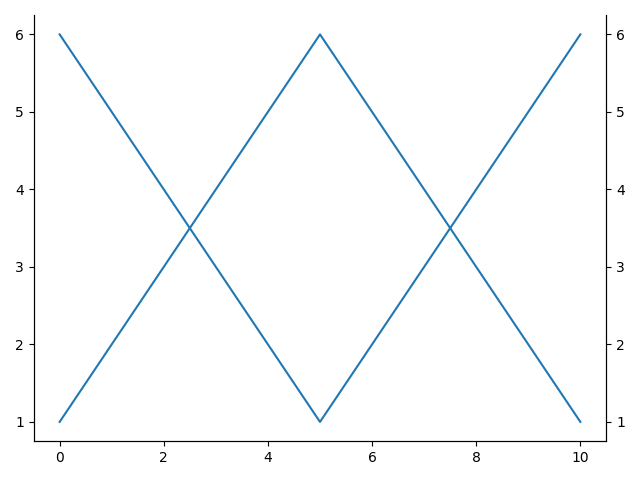
Plot data in 2 Y axes.

>>> import openhdemg.library as emg
>>> import matplotlib.pyplot as plt
>>> fig, ax1 = plt.subplots()
>>> ax1.plot([1, 2, 3, 4, 5, 6, 5, 4, 3, 2, 1])
>>> ax2 = ax1.twinx()
>>> ax2.plot([6, 5, 4, 3, 2, 1, 2, 3, 4, 5, 6])

Declare custom user plotting kwargs.

>>> line2d_kwargs_ax1 = {
...     "linewidth": 3,
...     "alpha": 0.2,
... }
>>> line2d_kwargs_ax2 = {
...     "linewidth": 1,
...     "alpha": 0.2,
...     "color": "red",
... }
>>> axes_kwargs = {
...     "grid": {
...         "visible": True,
...         "axis": "both",
...         "color": "gray",
...     },
... }

Merge default and user kwargs.

>>> fig_manager = emg.Figure_Layout_Manager(figure=fig)
>>> final_kwargs = fig_manager.get_final_kwargs(
...     line2d_kwargs_ax1=line2d_kwargs_ax1,
...     line2d_kwargs_ax2=line2d_kwargs_ax2,
...     axes_kwargs=axes_kwargs,
... )

Print them in an easy-to-read way.

>>> import pprint
>>> pp = pprint.PrettyPrinter(indent=4, width=40)
>>> pp.pprint(final_kwargs[0])
{   'alpha': 0.2,
    'linewidth': 3}

>>> pp.pprint(final_kwargs[1])
{   'alpha': 0.2,
    'color': 'red',
    'linewidth': 1}

>>> pp.pprint(final_kwargs[2])
{   'grid': {   'alpha': 0.7,
                'axis': 'both',
                'color': 'gray',
                'linestyle': '--',
                'linewidth': 0.5,
                'visible': True},
    'labels': {   'labelpad': 6,
                'title': None,
                'title_color': 'black',
                'title_pad': 14,
                'title_size': 12,
                'xlabel': None,
                'xlabel_color': 'black',
                'xlabel_size': 12,
                'ylabel_dx': None,
                'ylabel_dx_color': 'black',
                'ylabel_dx_size': 12,
                'ylabel_sx': None,
                'ylabel_sx_color': 'black',
                'ylabel_sx_size': 12},
    'ticks_ax1': {   'axis': 'both',
                    'colors': 'black',
                    'direction': 'out',
                    'labelrotation': 0,
                    'labelsize': 10},
    'ticks_ax2': {   'axis': 'y',
                    'colors': 'black',
                    'direction': 'out',
                    'labelrotation': 0,
                    'labelsize': 10}}

set_layout(tight_layout=True, despine='box')

Despine and show plots with a tight layout.

This method is called by the various plot functions contained in the library but can also be used by the user to quickly adjust the layout of custom plots.

PARAMETER	DESCRIPTION
tight_layout	If true, plt.tight_layout() is applied to the figure. TYPE: bool DEFAULT: True
despined	box No side is despined. all All the sides are despined. 1yaxis Right and top are despined. This is used to show the Y axis on the left side. 2yaxes Only the top is despined. This is used to show Y axes both on the left and right side at the same time. TYPE: str {"box", "all", "1yaxis", "2yaxes"} DEFAULT: "box"

Examples:

Plot data in 2 Y axes.

>>> import openhdemg.library as emg
>>> import matplotlib.pyplot as plt
>>> fig, ax1 = plt.subplots()
>>> ax1.plot([1, 2, 3, 4, 5, 6, 5, 4, 3, 2, 1])
>>> ax2 = ax1.twinx()
>>> ax2.plot([6, 5, 4, 3, 2, 1, 2, 3, 4, 5, 6])

Show the figure with 2 Y axes.

>>> fig_manager = emg.Figure_Layout_Manager(figure=fig)
>>> fig_manager.set_layout(tight_layout=True, despine="2yaxes")
>>> plt.show()

set_style_from_kwargs()

Set the style of the figure.

This method updates the main figure with the user-specified custom style, or with the standard openhdemg style if no style kwargs have been set with emg.Figure_Layout_Manager(figure).get_final_kwargs().

Examples:

Plot data in 2 Y axes.

>>> import openhdemg.library as emg
>>> import matplotlib.pyplot as plt
>>> fig, ax1 = plt.subplots()
>>> ax1.plot([1, 2, 3, 4, 5, 6, 5, 4, 3, 2, 1])
>>> ax2 = ax1.twinx()
>>> ax2.plot([6, 5, 4, 3, 2, 1, 2, 3, 4, 5, 6])

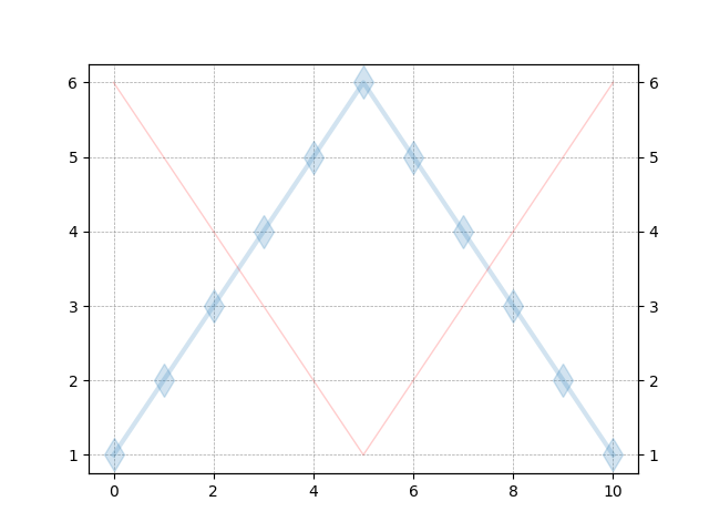
Declare custom user plotting kwargs.

>>> line2d_kwargs_ax1 = {
...     "linewidth": 3,
...     "alpha": 0.2,
...     "marker": "d",
...     "markersize": 15,
... }
>>> line2d_kwargs_ax2 = {
...     "linewidth": 1,
...     "alpha": 0.2,
...     "color": "red",
... }
>>> axes_kwargs = {
...     "grid": {
...         "visible": True,
...         "axis": "both",
...         "color": "gray",
...     },
... }

Merge default and user kwargs.

>>> fig_manager = emg.Figure_Layout_Manager(figure=fig)
>>> final_kwargs = fig_manager.get_final_kwargs(
...     line2d_kwargs_ax1=line2d_kwargs_ax1,
...     line2d_kwargs_ax2=line2d_kwargs_ax2,
...     axes_kwargs=axes_kwargs,
... )

Apply the custom style.

>>> fig_manager.set_style_from_kwargs()

Show the figure.

>>> plt.show()

Figure_Subplots_Layout_Manager

Class managing custom layout and custom settings for figures with multiple 2D subplots.

PARAMETER	DESCRIPTION
figure	The matplotlib.pyplot figure to manage. TYPE: pyplot `~.figure.Figure`

ATTRIBUTE	DESCRIPTION
figure	The managed matplotlib.pyplot figure. TYPE: pyplot `~.figure.Figure`

METHOD	DESCRIPTION
set_layout	Despine and show plots with a tight layout.
set_line2d_from_kwargs	Set line2d parameters from user kwargs.

Examples:

Initialise the Figure_Layout_Manager.

>>> import openhdemg.library as emg
>>> import matplotlib.pyplot as plt
>>> fig, axes = plt.subplots(nrows=5, ncols=5)
>>> fig_manager = emg.Figure_Subplots_Layout_Manager(figure=fig)

set_layout(tight_layout=True, despine='box')

Despine and show plots with a tight layout.

This method is called by the various plot functions contained in the library but can also be used by the user to quickly adjust the layout of custom plots.

PARAMETER	DESCRIPTION
tight_layout	If true, plt.tight_layout() is applied to the figure. TYPE: bool DEFAULT: True
despined	box No side is despined. all All the sides are despined. 1yaxis Right and top are despined. This is used to show the Y axis on the left side. 2yaxes Only the top is despined. This is used to show Y axes both on the left and right side at the same time. TYPE: str {"box", "all", "1yaxis", "2yaxes"} DEFAULT: "box"

Examples:

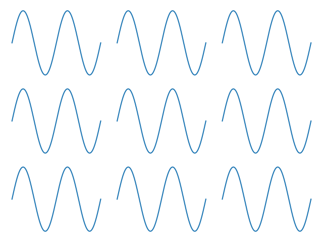
Plot sine waves in a 3x3 grid of subplots.

>>> import openhdemg.library as emg
>>> import matplotlib.pyplot as plt
>>> import numpy as np
>>> fig, axes = plt.subplots(nrows=3, ncols=3)
>>> x = np.linspace(0, 4 * np.pi, 500)
>>> base_signal = np.sin(x)
>>> for row in axes:
>>>     for ax in row:
>>>         ax.plot(x, base_signal)
>>>         ax.set_xticks([])
>>>         ax.set_yticks([])

Despine the figure and apply a tight layout.

>>> fig_manager = emg.Figure_Subplots_Layout_Manager(figure=fig)
>>> fig_manager.set_layout(tight_layout=True, despine="all")
>>> plt.show()

set_line2d_from_kwargs(line2d_kwargs_ax1=None)

Set the line2d style of the figure.

This method updates the main figure with the user-specified custom line2d style.

PARAMETER	DESCRIPTION
line2d_kwargs_ax1	User-specified keyword arguments for sets of Line2D objects. This can be a list of dictionaries containing the kwargs for each Line2D, or a single dictionary. If a single dictionary is passed, the same style will be applied to all the lines. TYPE: dict or list DEFAULT: None

Notes

line2d_kwargs_ax1 can contain any of the matplotlib.lines.Line2D parameters as described at: (https://matplotlib.org/stable/api/_as_gen/matplotlib.lines.Line2D.html).

Examples:

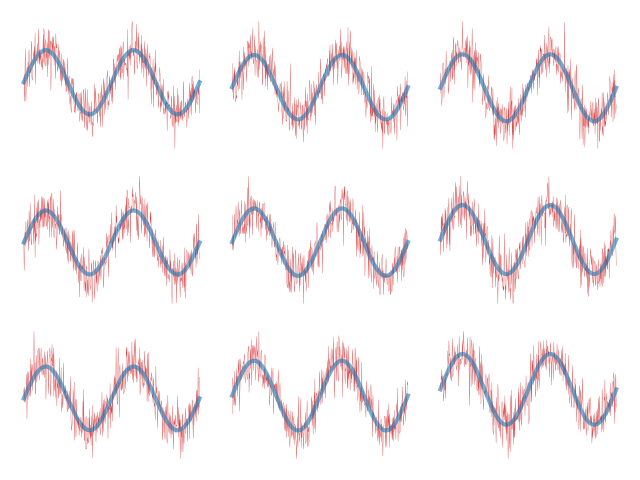
Plot sine waves in a 3x3 grid of subplots with and without noise.

>>> import openhdemg.library as emg
>>> import matplotlib.pyplot as plt
>>> import numpy as np
>>> fig, axes = plt.subplots(nrows=3, ncols=3)
>>> x = np.linspace(0, 4 * np.pi, 500)
>>> base_signal = np.sin(x)
>>> for row in axes:
>>>     for ax in row:
>>>         noisy_signal = base_signal + np.random.normal(
...             scale=0.4, size=base_signal.shape,
...         )
>>>         ax.plot(x, noisy_signal)
>>>         ax.plot(x, base_signal)
>>>         ax.set_xticks([])
>>>         ax.set_yticks([])

Set up the layout manager with custom styling for the 2 line2D (relative to the signal with and without noise, respectively).

>>> line2d_kwargs_ax1 = [
...     {
...         "color": "tab:red",
...         "alpha": 1,
...         "linewidth": 0.2,
...     },
...     {
...         "color": "tab:blue",
...         "linewidth": 3,
...         "alpha": 0.6,
...     },
... ]
>>> fig_manager = emg.Figure_Subplots_Layout_Manager(figure=fig)
>>> fig_manager.set_layout(despine="all")
>>> fig_manager.set_line2d_from_kwargs(
...     line2d_kwargs_ax1=line2d_kwargs_ax1,
... )
>>> plt.show()

plot_emgsig(emgfile, channels, manual_offset=0, addrefsig=False, timeinseconds=True, figsize=[20, 15], tight_layout=True, line2d_kwargs_ax1=None, line2d_kwargs_ax2=None, axes_kwargs=None, showimmediately=True)

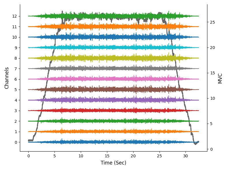
Plot the RAW_SIGNAL. Single or multiple channels.

Up to 12 channels (a common matrix row) can be easily observed togheter, but more can be plotted.

PARAMETER	DESCRIPTION
emgfile	The dictionary containing the emgfile. TYPE: dict
channels	The channel (int) or channels (list of int) to plot. The list can be passed as a manually-written list or with: channels=[*range(0, 13)]. We need the " * " operator to unpack the results of range into a list. channels is expected to be with base 0 (i.e., the first channel in the file is the number 0). TYPE: int or list
manual_offset	This parameter sets the scaling of the channels. If 0 (default), the channels' amplitude is scaled automatically to fit the plotting window. If > 0, the channels will be scaled based on the specified value. TYPE: int or float DEFAULT: 0
addrefsig	If True, the REF_SIGNAL is plotted in front of the signal with a separated y-axes. TYPE: bool DEFAULT: True
timeinseconds	Whether to show the time on the x-axes in seconds (True) or in samples (False). TYPE: bool DEFAULT: True
figsize	Size of the figure in centimeters [width, height]. TYPE: list DEFAULT: [20, 15]
tight_layout	If True (default), the plt.tight_layout() is called and the figure's layout is improved. It is useful to set it to False when calling the function from a GUI. TYPE: bool DEFAULT: True
line2d_kwargs_ax1	Kwargs for matplotlib.lines.Line2D relative to figure's axis 1 (the EMG signal). TYPE: dict DEFAULT: None
line2d_kwargs_ax2	Kwargs for matplotlib.lines.Line2D relative to figure's axis 2 (the reference signal). TYPE: dict DEFAULT: None
axes_kwargs	Kwargs for figure's axes. TYPE: dict DEFAULT: None
showimmediately	If True (default), plt.show() is called and the figure showed to the user. It is useful to set it to False when calling the function from a GUI. TYPE: bool DEFAULT: True

RETURNS	DESCRIPTION
fig	TYPE: pyplot `~.figure.Figure`

See also

• plot_differentials : plot the differential derivation of the RAW_SIGNAL by matrix column.

Examples:

Plot channels 0 to 12 and overlay the reference signal.

>>> import openhdemg.library as emg
>>> emgfile = emg.emg_from_samplefile()
>>> emg.plot_emgsig(
...     emgfile=emgfile,
...     channels=[*range(0,13)],
...     addrefsig=True,
...     timeinseconds=True,
...     figsize=[20, 15],
... )

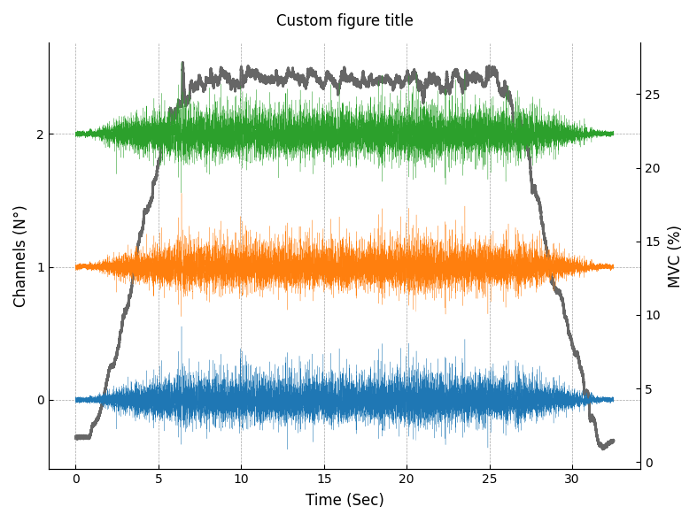
Plot channels and the reference signal with a custom look.

>>> import openhdemg.library as emg
>>> line2d_kwargs_ax1 = {
...     "linewidth": 0.2,
...     "alpha": 1,
... }
>>> line2d_kwargs_ax2 = {
...     "linewidth": 2,
...     "color": '0.4',
...     "alpha": 1,
... }
>>> axes_kwargs = {
...     "grid": {
...         "visible": True,
...         "axis": "both",
...         "color": "gray",
...         "linestyle": "--",
...         "linewidth": 0.5,
...         "alpha": 0.7
...     },
...     "labels": {
...         "xlabel": None,
...         "ylabel_sx": "Channels (N°)",
...         "ylabel_dx": "MVC (%)",
...         "title": "Custom figure title",
...         "xlabel_size": 12,
...         "xlabel_color": "black",
...         "ylabel_sx_size": 12,
...         "ylabel_sx_color": "black",
...         "ylabel_dx_size": 12,
...         "ylabel_dx_color": "black",
...         "labelpad": 6,
...         "title_size": 12,
...         "title_color": "black",
...         "title_pad": 14,
...     },
...     "ticks_ax1": {
...         "axis": "both",
...         "labelsize": 10,
...         "labelrotation": 0,
...         "direction": "in",
...         "colors": "black",
...     },
...     "ticks_ax2": {
...         "axis": "y",
...         "labelsize": 10,
...         "labelrotation": 0,
...         "direction": "in",
...         "colors": "black",
...     }
... }
>>> emgfile = emg.emg_from_samplefile()
>>> fig = emg.plot_emgsig(
...     emgfile,
...     channels=[*range(0, 3)],
...     manual_offset=0,
...     addrefsig=True,
...     timeinseconds=True,
...     tight_layout=True,
...     line2d_kwargs_ax1=line2d_kwargs_ax1,
...     line2d_kwargs_ax2=line2d_kwargs_ax2,
...     axes_kwargs=axes_kwargs,
...     showimmediately=True,
... )

plot_differentials(emgfile, differential, column='col0', manual_offset=0, addrefsig=False, timeinseconds=True, figsize=[20, 15], tight_layout=True, line2d_kwargs_ax1=None, line2d_kwargs_ax2=None, axes_kwargs=None, showimmediately=True)

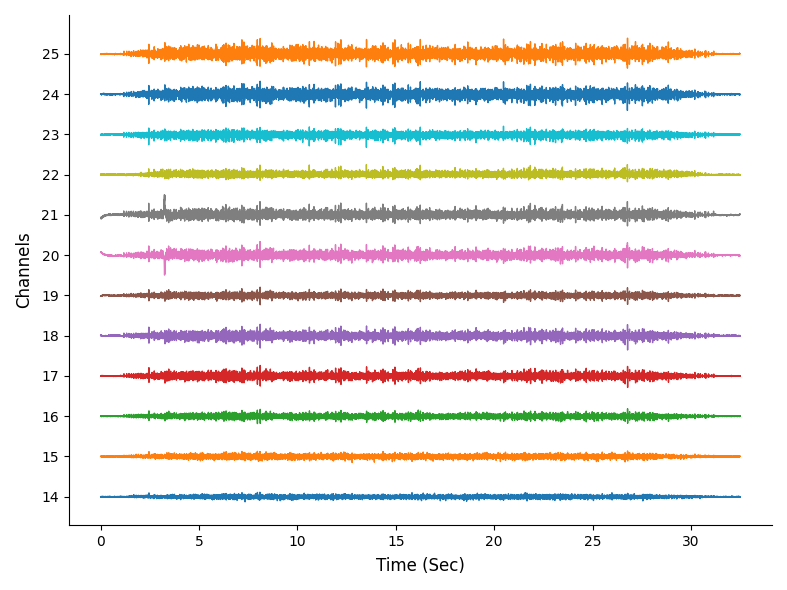
Plot the differential derivation of the RAW_SIGNAL by matrix column.

Both the single and the double differencials can be plotted. This function is used to plot also the sorted RAW_SIGNAL.

PARAMETER	DESCRIPTION
emgfile	The dictionary containing the original emgfile. TYPE: dict
differential	The dictionary containing the differential derivation of the RAW_SIGNAL. TYPE: dict
column	The matrix column to plot. Options are usyally "col0", "col1", "col2", "col3", "col4". but might change based on the size of the matrix used. TYPE: str {"col0", "col1", "col2", "col3", "col4", ...} DEFAULT: "col0"
manual_offset	This parameter sets the scaling of the channels. If 0 (default), the channels' amplitude is scaled automatically to fit the plotting window. If > 0, the channels will be scaled based on the specified value. TYPE: int or float DEFAULT: 0
addrefsig	If True, the REF_SIGNAL is plotted in front of the signal with a separated y-axes. TYPE: bool DEFAULT: True
timeinseconds	Whether to show the time on the x-axes in seconds (True) or in samples (False). TYPE: bool DEFAULT: True
figsize	Size of the figure in centimeters [width, height]. TYPE: list DEFAULT: [20, 15]
tight_layout	If True (default), the plt.tight_layout() is called and the figure's layout is improved. It is useful to set it to False when calling the function from a GUI. TYPE: bool DEFAULT: True
line2d_kwargs_ax1	Kwargs for matplotlib.lines.Line2D relative to figure's axis 1 (the EMG signal). TYPE: dict DEFAULT: None
line2d_kwargs_ax2	Kwargs for matplotlib.lines.Line2D relative to figure's axis 2 (the reference signal). TYPE: dict DEFAULT: None
axes_kwargs	Kwargs for figure's axes. TYPE: dict DEFAULT: None
showimmediately	If True (default), plt.show() is called and the figure showed to the user. It is useful to set it to False when calling the function from a GUI. TYPE: bool DEFAULT: True

RETURNS	DESCRIPTION
fig	TYPE: pyplot `~.figure.Figure`

See also

• diff : calculate single differential of RAW_SIGNAL on matrix rows.
• double_diff : calculate double differential of RAW_SIGNAL on matrix rows.
• plot_emgsig : pot the RAW_SIGNAL. Single or multiple channels.

Examples:

Plot the differential derivation of the second matrix column (col1).

>>> import openhdemg.library as emg
>>> emgfile = emg.emg_from_samplefile()
>>> sorted_rawemg = emg.sort_rawemg(
...     emgfile=emgfile,
...     code="GR08MM1305",
...     orientation=180,
... )
>>> sd=emg.diff(sorted_rawemg=sorted_rawemg)
>>> emg.plot_differentials(
...     emgfile=emgfile,
...     differential=sd,
...     column="col1",
...     addrefsig=False,
...     timeinseconds=True,
...     figsize=[20, 15],
...     showimmediately=True,
... )

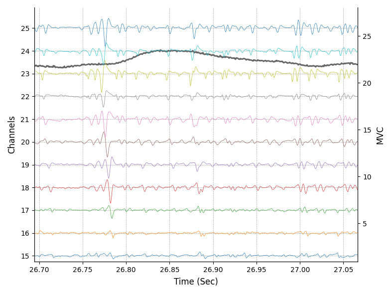
Plot the double differential derivation of the second matrix column (col1) with custom styles (the graph shows a zoomed section).

>>> import openhdemg.library as emg
>>> emgfile = emg.emg_from_samplefile()
>>> sorted_rawemg = emg.sort_rawemg(
...     emgfile=emgfile,
...     code="GR08MM1305",
...     orientation=180,
... )
>>> sd=emg.double_diff(sorted_rawemg=sorted_rawemg)
>>> line2d_kwargs_ax1 = {"linewidth": 0.5}
>>> axes_kwargs = {
...     "grid": {
...         "visible": True,
...         "axis": "both",
...         "color": "gray",
...         "linestyle": "--",
...         "linewidth": 0.5,
...         "alpha": 0.7
...     },
... }
>>> fig = emg.plot_differentials(
...     emgfile,
...     differential=sd,
...     column="col1",
...     manual_offset=1000,
...     addrefsig=True,
...     timeinseconds=True,
...     tight_layout=True,
...     line2d_kwargs_ax1=line2d_kwargs_ax1,
...     axes_kwargs=axes_kwargs,
...     showimmediately=True,
... )

For further examples on how to customise the figure's layout, refer to plot_emgsig().

plot_refsig(emgfile, ylabel='', timeinseconds=True, figsize=[20, 15], tight_layout=True, line2d_kwargs_ax1=None, axes_kwargs=None, showimmediately=True)

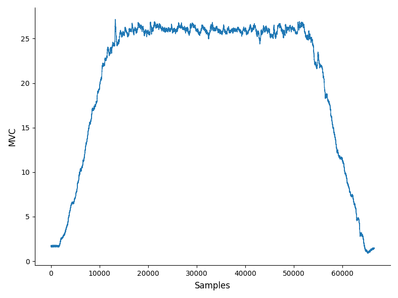
Plot the REF_SIGNAL.

The REF_SIGNAL is usually expressed as % MVC for submaximal contractions or as Kilograms (Kg) or Newtons (N) for maximal contractions, but any value can be plotted.

PARAMETER	DESCRIPTION
emgfile	The dictionary containing the emgfile. TYPE: dict
ylabel	WARNING! This parameter is deprecated since v0.1.1 and will be removed after v0.2.0. Please use axes_kwargs instead. See examples in the plot_refsig documentation. TYPE: str DEFAULT: ''
timeinseconds	Whether to show the time on the x-axes in seconds (True) or in samples (False). TYPE: bool DEFAULT: True
figsize	Size of the figure in centimeters [width, height]. TYPE: list DEFAULT: [20, 15]
tight_layout	If True (default), the plt.tight_layout() is called and the figure's layout is improved. It is useful to set it to False when calling the function from a GUI. TYPE: bool DEFAULT: True
line2d_kwargs_ax1	Kwargs for matplotlib.lines.Line2D relative to figure's axis 1 (the reference signal). TYPE: dict DEFAULT: None
axes_kwargs	Kwargs for figure's axes. TYPE: dict DEFAULT: None
showimmediately	If True (default), plt.show() is called and the figure showed to the user. It is useful to set it to False when calling the function from a GUI. TYPE: bool DEFAULT: True

RETURNS	DESCRIPTION
fig	TYPE: pyplot `~.figure.Figure`

Examples:

Plot the reference signal.

>>> import openhdemg.library as emg
>>> emgfile = emg.emg_from_samplefile()
>>> emg.plot_refsig(emgfile=emgfile)

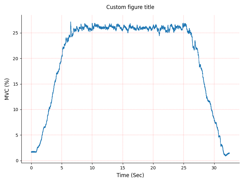
Plot the reference signal with custom labels and style.

>>> import openhdemg.library as emg
>>> emgfile = emg.emg_from_samplefile()
>>> line2d_kwargs_ax1 = {"linewidth": 1}
>>> axes_kwargs = {
...     "grid": {
...         "visible": True,
...         "axis": "both",
...         "color": "red",
...         "linestyle": "--",
...         "linewidth": 0.3,
...         "alpha": 0.7
...     },
...     "labels": {
...         "ylabel_sx": "MVC (%)",
...         "title": "Custom figure title",
...     },
... }
>>> fig = emg.plot_refsig(
...     emgfile,
...     timeinseconds=True,
...     tight_layout=True,
...     line2d_kwargs_ax1=line2d_kwargs_ax1,
...     axes_kwargs=axes_kwargs,
...     showimmediately=True,
... )

plot_mupulses(emgfile, munumber='all', linewidths=0, linelengths=0.9, addrefsig=True, timeinseconds=True, figsize=[20, 15], tight_layout=True, line2d_kwargs_ax1=None, line2d_kwargs_ax2=None, axes_kwargs=None, showimmediately=True)

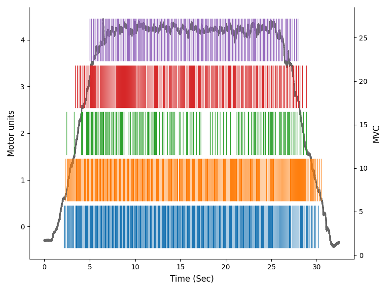
Plot the MUPULSES (binary representation of the firings time).

PARAMETER	DESCRIPTION
emgfile	The dictionary containing the emgfile. TYPE: dict
munumber	all IPTS of all the MUs is plotted. Otherwise, a single MU (int) or multiple MUs (list of int) can be specified. The list can be passed as a manually-written list or with: munumber=[*range(0, n)]. We need the " * " operator to unpack the results of range into a list. munumber is expected to be with base 0 (i.e., the first MU in the file is the number 0). TYPE: (str, int or list) DEFAULT: "all"
linewidths	WARNING! This parameter is deprecated since v0.1.1 and will be removed after v0.2.0. Please use line2d_kwargs_ax1 instead. See examples in the plot_mupulses documentation. TYPE: float DEFAULT: 0
linelengths	The vertical length of each line. This must be a value between 0 and 1. TYPE: float DEFAULT: 0.9
addrefsig	If True, the REF_SIGNAL is plotted in front of the MUs pulses with a separated y-axes. TYPE: bool DEFAULT: True
timeinseconds	Whether to show the time on the x-axes in seconds (True) or in samples (False). TYPE: bool DEFAULT: True
figsize	Size of the figure in centimeters [width, height]. TYPE: list DEFAULT: [20, 15]
tight_layout	If True (default), the plt.tight_layout() is called and the figure's layout is improved. It is useful to set it to False when calling the function from a GUI. TYPE: bool DEFAULT: True
line2d_kwargs_ax1	Kwargs for matplotlib.lines.Line2D relative to figure's axis 1 (the MUPULSES). TYPE: dict DEFAULT: None
line2d_kwargs_ax2	Kwargs for matplotlib.lines.Line2D relative to figure's axis 2 (the reference signal). TYPE: dict DEFAULT: None
axes_kwargs	Kwargs for figure's axes. TYPE: dict DEFAULT: None
showimmediately	If True (default), plt.show() is called and the figure showed to the user. It is useful to set it to False when calling the function from a GUI. TYPE: bool DEFAULT: True

RETURNS	DESCRIPTION
fig	TYPE: pyplot `~.figure.Figure`

See also

• plot_ipts : plot the MUs impulse train per second (IPTS).
• plot_idr : plot the instantaneous discharge rate.

Examples:

Plot MUs pulses based on recruitment order and overlay the reference signal.

>>> import openhdemg.library as emg
>>> emgfile = emg.emg_from_samplefile()
>>> emgfile = emg.sort_mus(emgfile)
>>> emg.plot_mupulses(
...     emgfile=emgfile,
...     addrefsig=True,
...     timeinseconds=True,
...     figsize=[20, 15],
...     showimmediately=True,
... )

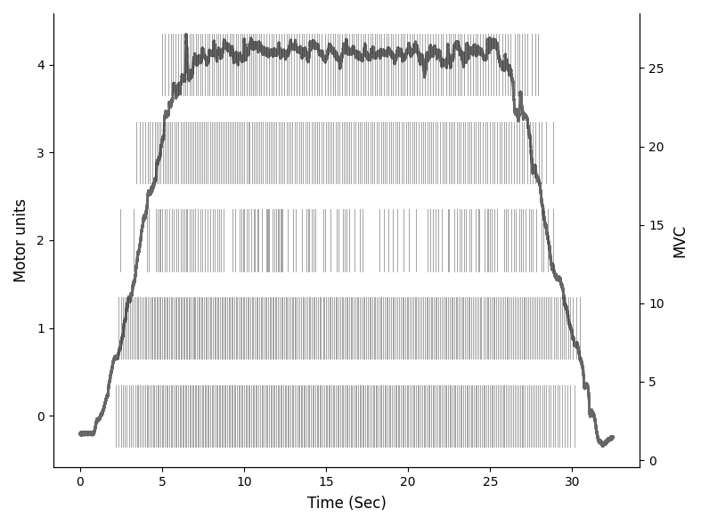
Plot MUs pulses based on recruitment order and adjust lines width, color and length.

>>> import openhdemg.library as emg
>>> emgfile = emg.emg_from_samplefile()
>>> emgfile = emg.sort_mus(emgfile)
>>> line2d_kwargs_ax1 = {
...     "linewidth": 0.7,
...     "color": "0.1",
...     "alpha": 0.4,
... }
>>> fig = emg.plot_mupulses(
...     emgfile,
...     munumber="all",
...     linelengths=0.7,
...     addrefsig=True,
...     timeinseconds=True,
...     tight_layout=True,
...     line2d_kwargs_ax1=line2d_kwargs_ax1,
...     showimmediately=True,
... )

For further examples on how to customise the figure's layout, refer to plot_emgsig().

plot_ipts(emgfile, munumber='all', addrefsig=False, timeinseconds=True, figsize=[20, 15], tight_layout=True, line2d_kwargs_ax1=None, line2d_kwargs_ax2=None, axes_kwargs=None, showimmediately=True)

Plot the IPTS (decomposed source).

IPTS is the non-binary representation of the MUs firing times.

PARAMETER	DESCRIPTION
emgfile	The dictionary containing the emgfile. TYPE: dict
munumber	all IPTS of all the MUs is plotted. Otherwise, a single MU (int) or multiple MUs (list of int) can be specified. The list can be passed as a manually-written list or with: munumber=[*range(0, 12)]. We need the " * " operator to unpack the results of range into a list. munumber is expected to be with base 0 (i.e., the first MU in the file is the number 0). TYPE: (str, int or list) DEFAULT: "all"
addrefsig	If True, the REF_SIGNAL is plotted in front of the signal with a separated y-axes. TYPE: bool DEFAULT: True
timeinseconds	Whether to show the time on the x-axes in seconds (True) or in samples (False). TYPE: bool DEFAULT: True
figsize	Size of the figure in centimeters [width, height]. TYPE: list DEFAULT: [20, 15]
tight_layout	If True (default), the plt.tight_layout() is called and the figure's layout is improved. It is useful to set it to False when calling the function from a GUI. TYPE: bool DEFAULT: True
line2d_kwargs_ax1	Kwargs for matplotlib.lines.Line2D relative to figure's axis 1 (the IPTS). TYPE: dict DEFAULT: None
line2d_kwargs_ax2	Kwargs for matplotlib.lines.Line2D relative to figure's axis 2 (the reference signal). TYPE: dict DEFAULT: None
axes_kwargs	Kwargs for figure's axes. TYPE: dict DEFAULT: None
showimmediately	If True (default), plt.show() is called and the figure showed to the user. It is useful to set it to False when calling the function from a GUI. TYPE: bool DEFAULT: True

RETURNS	DESCRIPTION
fig	TYPE: pyplot `~.figure.Figure`

See also

• plot_mupulses : plot the binary representation of the firings.
• plot_idr : plot the instantaneous discharge rate.

Notes

munumber = "all" corresponds to: munumber = [*range(0, emgfile["NUMBER_OF_MUS"])]

Examples:

Plot IPTS of all the MUs and overlay the reference signal.

>>> import openhdemg.library as emg
>>> emgfile = emg.emg_from_samplefile()
>>> emg.plot_ipts(
...     emgfile=emgfile,
...     munumber="all",
...     addrefsig=True,
...     timeinseconds=True,
...     figsize=[20, 15],
...     showimmediately=True,
... )

Plot IPTS of two MUs.

>>> import openhdemg.library as emg
>>> emgfile = emg.emg_from_samplefile()
>>> emg.plot_ipts(
...     emgfile=emgfile,
...     munumber=[1, 3],
...     addrefsig=False,
...     timeinseconds=True,
...     figsize=[20, 15],
...     showimmediately=True,
... )

Plot IPTS of all the MUs, the reference signal, smaller lines and a background grid.

>>> import openhdemg.library as emg
>>> emgfile = emg.emg_from_samplefile()
>>> line2d_kwargs_ax1 = {"linewidth": 0.5}
>>> axes_kwargs = {
...     "grid": {
...         "visible": True,
...         "axis": "both",
...         "color": "gray",
...         "linestyle": "--",
...         "linewidth": 1,
...         "alpha": 0.7
...     },
... }
>>> fig = emg.plot_ipts(
...     emgfile,
...     munumber="all",
...     addrefsig=True,
...     timeinseconds=True,
...     tight_layout=True,
...     axes_kwargs=axes_kwargs,
...     showimmediately=True,
... )

For additional examples on how to customise the figure's layout, refer to plot_emgsig().

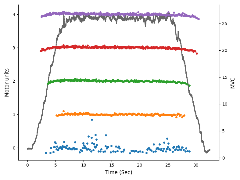
plot_idr(emgfile, munumber='all', addrefsig=True, timeinseconds=True, figsize=[20, 15], tight_layout=True, line2d_kwargs_ax1=None, line2d_kwargs_ax2=None, axes_kwargs=None, showimmediately=True)

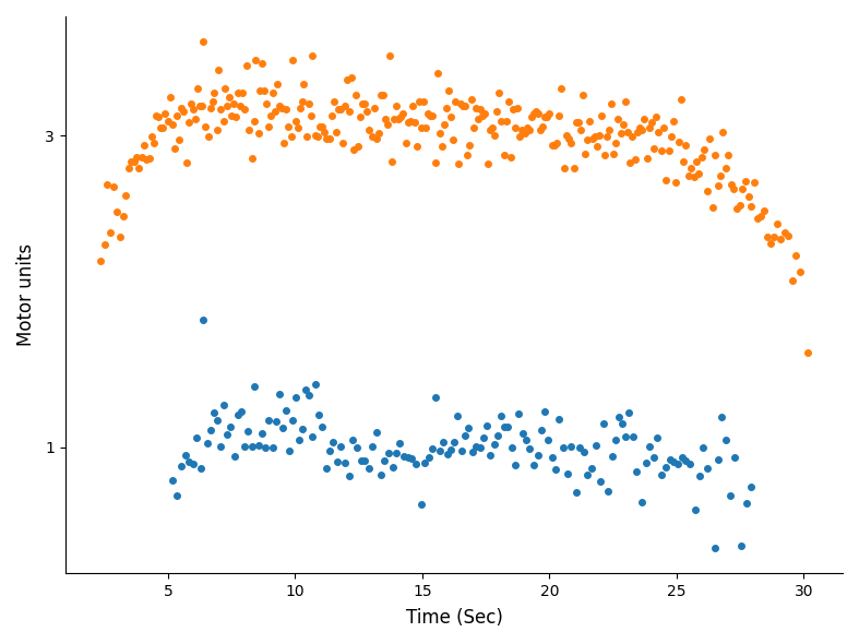
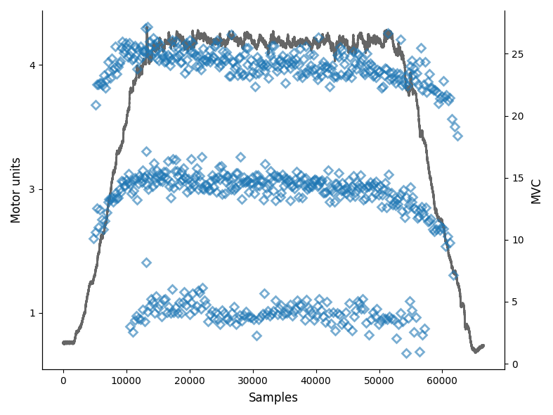
Plot the instantaneous discharge rate (IDR).

PARAMETER	DESCRIPTION
emgfile	The dictionary containing the emgfile. TYPE: dict
munumber	all IDR of all the MUs is plotted. Otherwise, a single MU (int) or multiple MUs (list of int) can be specified. The list can be passed as a manually-written list or with: munumber=[*range(0, 12)]. We need the " * " operator to unpack the results of range into a list. munumber is expected to be with base 0 (i.e., the first MU in the file is the number 0). TYPE: (str, int or list) DEFAULT: "all"
addrefsig	If True, the REF_SIGNAL is plotted in front of the MUs IDR with a separated y-axes. TYPE: bool DEFAULT: True
timeinseconds	Whether to show the time on the x-axes in seconds (True) or in samples (False). TYPE: bool DEFAULT: True
figsize	Size of the figure in centimeters [width, height]. TYPE: list DEFAULT: [20, 15]
tight_layout	If True (default), the plt.tight_layout() is called and the figure's layout is improved. It is useful to set it to False when calling the function from a GUI. TYPE: bool DEFAULT: True
line2d_kwargs_ax1	Kwargs for matplotlib.lines.Line2D relative to figure's axis 1 (the IDR). TYPE: dict DEFAULT: None
line2d_kwargs_ax2	Kwargs for matplotlib.lines.Line2D relative to figure's axis 2 (the reference signal). TYPE: dict DEFAULT: None
axes_kwargs	Kwargs for figure's axes. TYPE: dict DEFAULT: None
showimmediately	If True (default), plt.show() is called and the figure showed to the user. It is useful to set it to False when calling the function from a GUI. TYPE: bool DEFAULT: True

RETURNS	DESCRIPTION
fig	TYPE: pyplot `~.figure.Figure`

See also

• plot_mupulses : plot the binary representation of the firings.
• plot_ipts : plot the impulse train per second (IPTS).

Notes

munumber = "all" corresponds to munumber = [*range(0, emgfile["NUMBER_OF_MUS"])]

Examples:

Plot IDR of all the MUs and overlay the reference signal.

>>> import openhdemg.library as emg
>>> emgfile = emg.emg_from_samplefile()
>>> emg.plot_idr(
...     emgfile=emgfile,
...     munumber="all",
...     addrefsig=True,
...     timeinseconds=True,
...     figsize=[20, 15],
...     showimmediately=True,
... )

Plot IDR of two MUs.

>>> import openhdemg.library as emg
>>> emgfile = emg.emg_from_samplefile()
>>> emg.plot_idr(
...     emgfile=emgfile,
...     munumber=[1, 3],
...     addrefsig=False,
...     timeinseconds=True,
...     figsize=[20, 15],
...     showimmediately=True,
... )

Plot IDR and use custom markers.

>>> import openhdemg.library as emg
>>> emgfile = emg.emg_from_samplefile()
>>> line2d_kwargs_ax1 = {
...     "marker": "D",
...     "markersize": 6,
...     "markeredgecolor": "tab:blue",
...     "markeredgewidth": "2",
...     "fillstyle": "none",
...     "alpha": 0.6,
... }
>>> fig = emg.plot_idr(
...     emgfile,
...     munumber=[1, 3, 4],
...     addrefsig=True,
...     timeinseconds=False,
...     tight_layout=True,
...     line2d_kwargs_ax1=line2d_kwargs_ax1,
...     showimmediately=True,
... )

For additional examples on how to customise the figure's layout, refer to plot_emgsig().

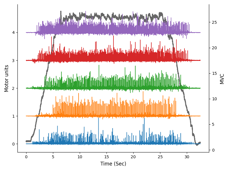
plot_smoothed_dr(emgfile, smoothfits, munumber='all', addidr=True, stack=True, addrefsig=True, timeinseconds=True, figsize=[20, 15], tight_layout=True, line2d_kwargs_ax1=None, line2d_kwargs_ax2=None, axes_kwargs=None, showimmediately=True)

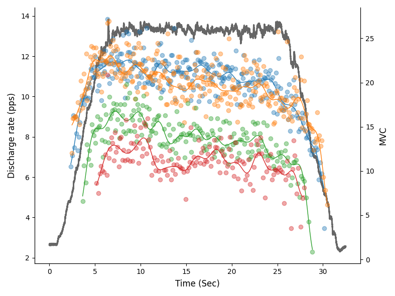
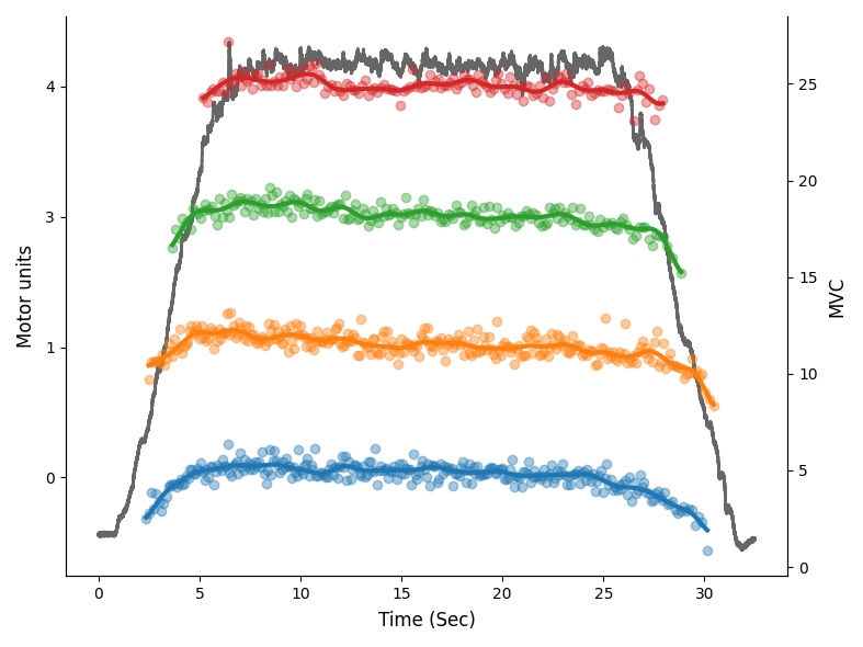
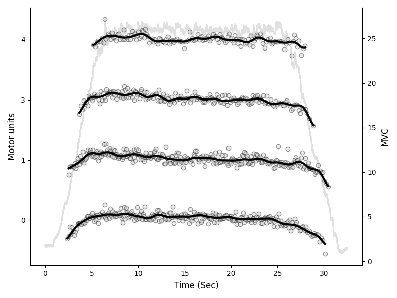
Plot the smoothed discharge rate.

PARAMETER	DESCRIPTION
emgfile	The dictionary containing the emgfile. TYPE: dict
smoothfits	Smoothed discharge rate estimates aligned in time. Columns should contain the smoothed discharge rate for each MU. TYPE: DataFrame
munumber	all IDR of all the MUs is plotted. Otherwise, a single MU (int) or multiple MUs (list of int) can be specified. The list can be passed as a manually-written list or with: munumber=[*range(0, 12)]. We need the " * " operator to unpack the results of range into a list. munumber is expected to be with base 0 (i.e., the first MU in the file is the number 0). TYPE: (str, int or list) DEFAULT: "all"
addidr	Whether to show also the IDR behind the smoothed DR line. TYPE: bool DEFAULT: True
stack	Whether to stack multiple MUs. If False, all the MUs smoothed DR will be plotted on the same line. TYPE: bool DEFAULT: True
addrefsig	If True, the REF_SIGNAL is plotted in front of the MUs IDR with a separated y-axes. TYPE: bool DEFAULT: True
timeinseconds	Whether to show the time on the x-axes in seconds (True) or in samples (False). TYPE: bool DEFAULT: True
figsize	Size of the figure in centimeters [width, height]. TYPE: list DEFAULT: [20, 15]
tight_layout	If True (default), the plt.tight_layout() is called and the figure's layout is improved. It is useful to set it to False when calling the function from a GUI. TYPE: bool DEFAULT: True
line2d_kwargs_ax1	Kwargs for matplotlib.lines.Line2D relative to figure's axis 1 (in this case, smoothfits and idr). TYPE: dict DEFAULT: None
line2d_kwargs_ax2	Kwargs for matplotlib.lines.Line2D relative to figure's axis 2 (the reference signal). TYPE: dict DEFAULT: None
axes_kwargs	Kwargs for figure's axes. TYPE: dict DEFAULT: None
showimmediately	If True (default), plt.show() is called and the figure showed to the user. It is useful to set it to False when calling the function from a GUI. TYPE: bool DEFAULT: True

RETURNS	DESCRIPTION
fig	TYPE: pyplot `~.figure.Figure`

See also

• compute_svr : Fit MU discharge rates with Support Vector Regression, nonlinear regression.

Notes

munumber = "all" corresponds to: munumber = [*range(0, emgfile["NUMBER_OF_MUS"])]

Examples:

Smooth MUs DR using Support Vector Regression. Plot the smoothed DR of some MUs and overlay the IDR and the reference signal.

>>> import openhdemg.library as emg
>>> import pandas as pd
>>> emgfile = emg.emg_from_samplefile()
>>> emgfile = emg.sort_mus(emgfile=emgfile)
>>> svrfits = emg.compute_svr(emgfile)
>>> smoothfits = pd.DataFrame(svrfits["gensvr"]).transpose()
>>> fig = emg.plot_smoothed_dr(
...     emgfile,
...     smoothfits=smoothfits,
...     munumber=[0, 1, 3, 4],
...     addidr=True,
...     stack=False,
...     addrefsig=True,
... )

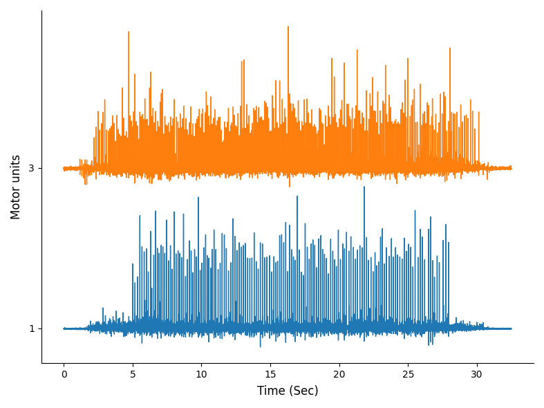
Stack the MUs and change line width.

>>> import openhdemg.library as emg
>>> import pandas as pd
>>> emgfile = emg.emg_from_samplefile()
>>> emgfile = emg.sort_mus(emgfile=emgfile)
>>> svrfits = emg.compute_svr(emgfile)
>>> smoothfits = pd.DataFrame(svrfits["gensvr"]).transpose()
>>> line2d_kwargs_ax1 = {
...     "linewidth": 3,
... }
>>> fig = emg.plot_smoothed_dr(
...     emgfile,
...     smoothfits=smoothfits,
...     munumber=[0, 1, 3, 4],
...     addidr=True,
...     stack=True,
...     addrefsig=True,
...     line2d_kwargs_ax1=line2d_kwargs_ax1,
... )

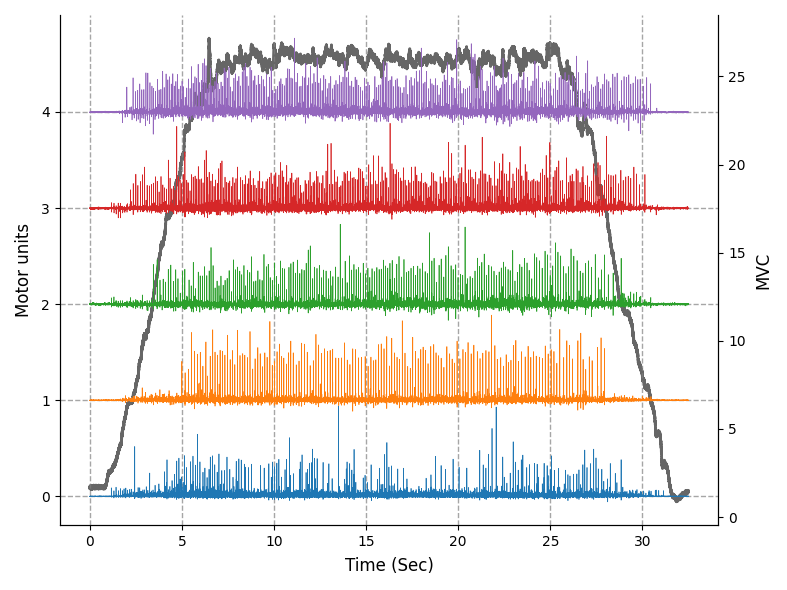
Plot in black and white.

>>> import openhdemg.library as emg
>>> import pandas as pd
>>> emgfile = emg.emg_from_samplefile()
>>> emgfile = emg.sort_mus(emgfile=emgfile)
>>> svrfits = emg.compute_svr(emgfile)
>>> smoothfits = pd.DataFrame(svrfits["gensvr"]).transpose()
>>> line2d_kwargs_ax1 = {
...     "linewidth": 3,
...     "markerfacecolor": "0.8",
...     "markeredgecolor": "k",
...     "color": "k",
... }
>>> line2d_kwargs_ax2 = {"alpha": 0.2}
>>> fig = emg.plot_smoothed_dr(
...     emgfile,
...     smoothfits=smoothfits,
...     munumber=[0, 1, 3, 4],
...     addidr=True,
...     stack=True,
...     addrefsig=True,
...     line2d_kwargs_ax1=line2d_kwargs_ax1,
...     line2d_kwargs_ax2=line2d_kwargs_ax2,
... )

For additional examples on how to customise the figure's layout, refer to plot_emgsig().

plot_muaps(sta_dict, title='MUAPs from STA', figsize=[20, 15], tight_layout=False, line2d_kwargs_ax1=None, showimmediately=True)

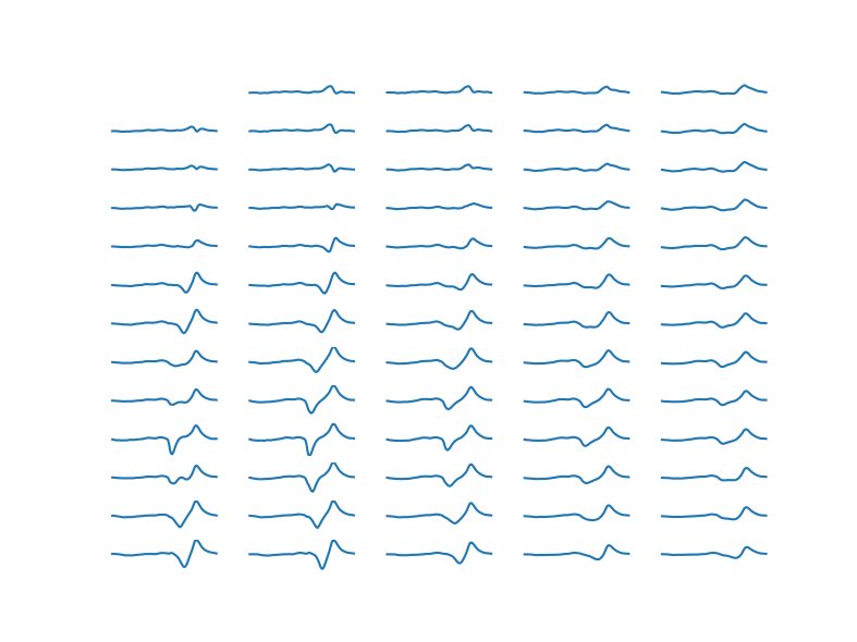
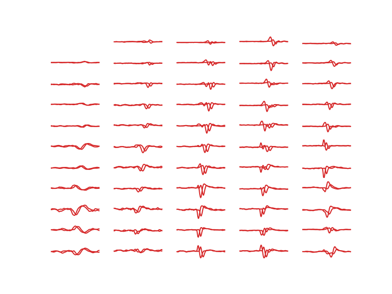
Plot MUAPs obtained from STA from one or multiple MUs.

PARAMETER	DESCRIPTION
sta_dict	dict containing STA of the specified MU or a list of dicts containing STA of specified MUs. If a list is passed, different MUs are overlayed. This is useful for visualisation of MUAPs during tracking or duplicates removal. TYPE: dict or list
title	Title of the plot. TYPE: str DEFAULT: "MUAPs from STA"
figsize	Size of the figure in centimeters [width, height]. TYPE: list DEFAULT: [20, 15]
tight_layout	If True (default), the plt.tight_layout() is called and the figure's layout is improved. It is useful to set it to False when calling the function from a GUI or if the final layout is not correct. TYPE: bool DEFAULT: False
line2d_kwargs_ax1	User-specified keyword arguments for sets of Line2D objects. This can be a list of dictionaries containing the kwargs for each Line2D, or a single dictionary. If a single dictionary is passed, the same style will be applied to all the lines. See examples. TYPE: dict or list DEFAULT: None
showimmediately	If True (default), plt.show() is called and the figure showed to the user. It is useful to set it to False when calling the function from a GUI. TYPE: bool DEFAULT: True

RETURNS	DESCRIPTION
fig	TYPE: pyplot `~.figure.Figure`

See also

• sta : computes the spike-triggered average (STA) of every MUs.
• plot_muap : for overplotting all the STAs and the average STA of a MU.
• align_by_xcorr : for alignin the STAs of two different MUs.

Notes

There is no limit to the number of MUs and STA files that can be overplotted.

Remember: the different STAs should be matched with same number of electrode, processing (i.e., differential) and computed on the same timewindow.

Examples:

Plot MUAPs of a single MU.

>>> import openhdemg.library as emg
>>> emgfile = emg.emg_from_samplefile()
>>> sorted_rawemg = emg.sort_rawemg(
...     emgfile=emgfile,
...     code="GR08MM1305",
...     orientation=180,
...     dividebycolumn=True,
... )
>>> sta = emg.sta(
...     emgfile=emgfile,
...     sorted_rawemg=sorted_rawemg,
...     firings="all",
...     timewindow=50,
... )
>>> emg.plot_muaps(sta_dict=sta[0])

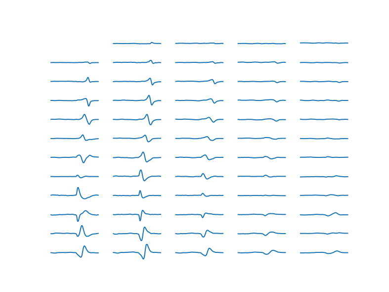
Plot single differential derivation MUAPs of a single MU.

>>> import openhdemg.library as emg
>>> emgfile = emg.emg_from_samplefile()
>>> sorted_rawemg = emg.sort_rawemg(
...     emgfile=emgfile,
...     code="GR08MM1305",
...     orientation=180,
...     dividebycolumn=True,
... )
>>> sorted_rawemg = emg.diff(sorted_rawemg=sorted_rawemg)
>>> sta = emg.sta(
...     emgfile=emgfile,
...     sorted_rawemg=sorted_rawemg,
...     firings="all",
...     timewindow=50,
... )
>>> emg.plot_muaps(sta_dict=sta[1])

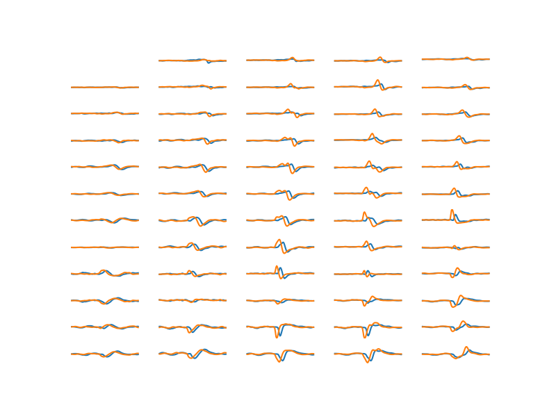
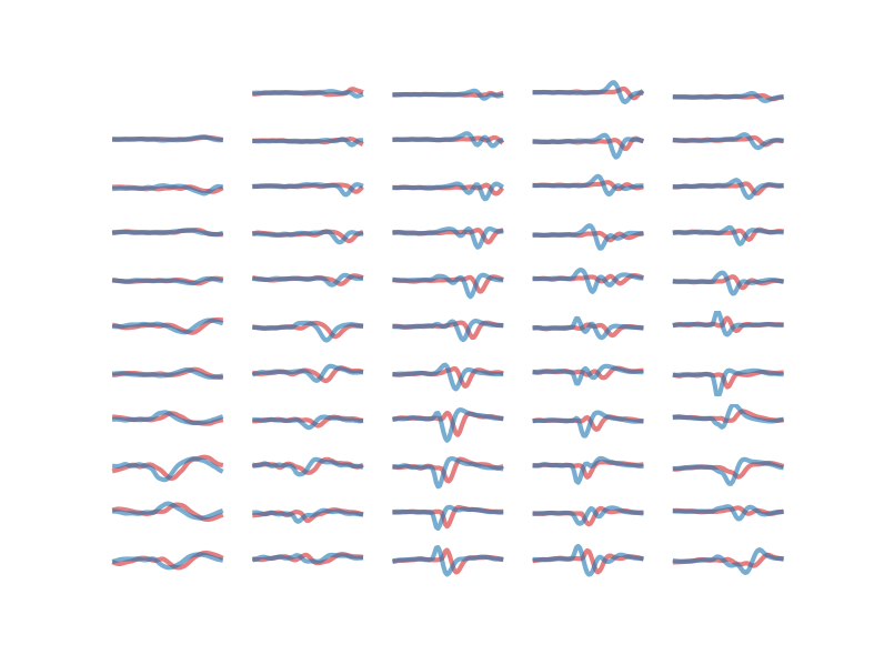
Plot single differential derivation MUAPs of two MUs from the same file.

>>> import openhdemg.library as emg
>>> emgfile = emg.emg_from_samplefile()
>>> sorted_rawemg = emg.sort_rawemg(
...     emgfile=emgfile,
...     code="GR08MM1305",
...     orientation=180,
...     dividebycolumn=True,
... )
>>> sorted_rawemg = emg.diff(sorted_rawemg=sorted_rawemg)
>>> sta = emg.sta(
...     emgfile=emgfile,
...     sorted_rawemg=sorted_rawemg,
...     firings="all",
...     timewindow=50,
... )
>>> emg.plot_muaps(sta_dict=[sta[2], sta[3]])

Plot double differential derivation MUAPs of two MUs from the same file and change their color.

>>> import openhdemg.library as emg
>>> emgfile = emg.emg_from_samplefile()
>>> sorted_rawemg = emg.sort_rawemg(
...     emgfile=emgfile,
...     code="GR08MM1305",
...     orientation=180,
...     dividebycolumn=True,
... )
>>> sorted_rawemg = emg.double_diff(sorted_rawemg=sorted_rawemg)
>>> sta = emg.sta(
...     emgfile=emgfile,
...     sorted_rawemg=sorted_rawemg,
...     firings="all",
...     timewindow=50,
... )
>>> line2d_kwargs_ax1 = {
...     "color": "tab:red",
... }
>>> emg.plot_muaps(
...     sta_dict=[sta[2], sta[3]],
...     line2d_kwargs_ax1=line2d_kwargs_ax1,
... )

Or change their color and style individually.

>>> import openhdemg.library as emg
>>> emgfile = emg.emg_from_samplefile()
>>> sorted_rawemg = emg.sort_rawemg(
...     emgfile=emgfile,
...     code="GR08MM1305",
...     orientation=180,
...     dividebycolumn=True,
... )
>>> sorted_rawemg = emg.double_diff(sorted_rawemg=sorted_rawemg)
>>> sta = emg.sta(
...     emgfile=emgfile,
...     sorted_rawemg=sorted_rawemg,
...     firings="all",
...     timewindow=30,
... )
>>> line2d_kwargs_ax1 = [
...     {
...         "color": "tab:red",
...         "linewidth": 3,
...         "alpha": 0.6,
...     },
...     {
...         "color": "tab:blue",
...         "linewidth": 3,
...         "alpha": 0.6,
...     },
... ]
>>> emg.plot_muaps(
...     sta_dict=[sta[2], sta[3]],
...     line2d_kwargs_ax1=line2d_kwargs_ax1,
... )

plot_muap(emgfile, stmuap, munumber, column, channel, channelprog=False, average=True, timeinseconds=True, figsize=[20, 15], tight_layout=True, line2d_kwargs_ax1=None, line2d_kwargs_ax2=None, axes_kwargs=None, showimmediately=True)

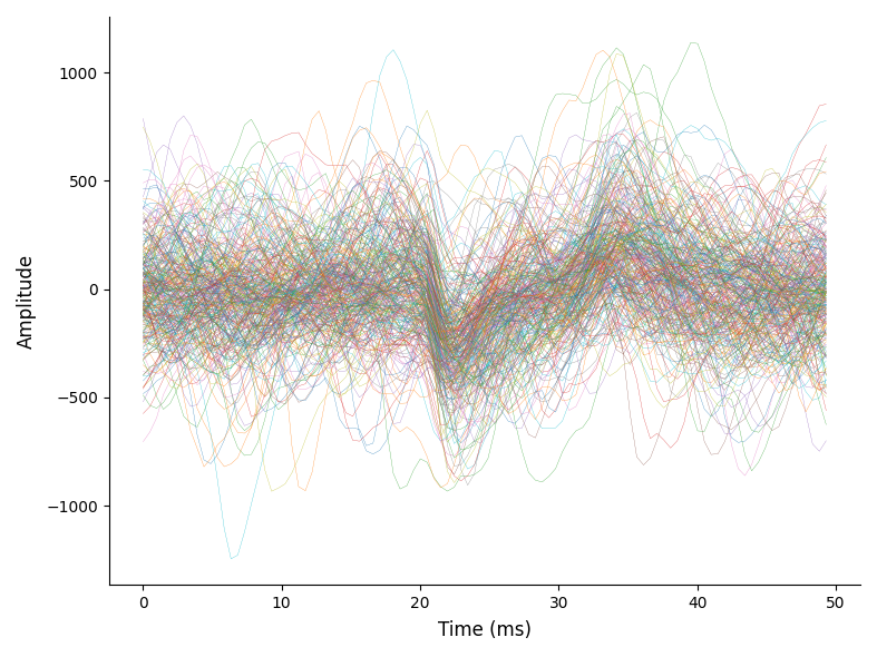
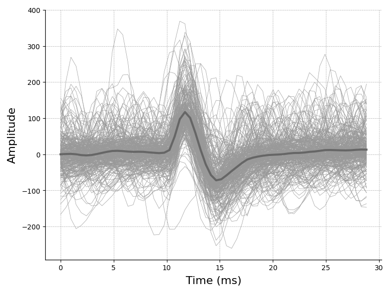
Plot the MUAPs of a specific matrix channel.

Plot the MUs action potential (MUAPs) shapes with or without average.

PARAMETER	DESCRIPTION
emgfile	The dictionary containing the emgfile. TYPE: dict
stmuap	dict containing a dict of ST MUAPs (pd.DataFrame) for every MUs. TYPE: dict
munumber	The number of the MU to plot. TYPE: int
column	The matrix columns. Options are usyally "col0", "col1", "col2", ..., last column. TYPE: str
channel	The channel of the matrix to plot. This can be the real channel number if channelprog=False (default), or a progressive number (from 0 to the length of the matrix column) if channelprog=True. TYPE: int
channelprog	Whether to use the real channel number or a progressive number (see channel). TYPE: bool DEFAULT: False
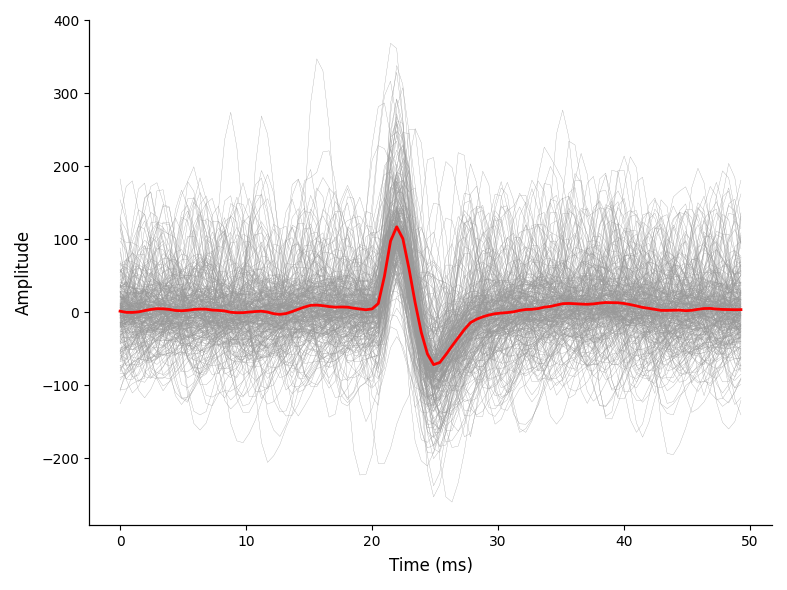
average	Whether to plot also the MUAPs average obtained by spike triggered average. TYPE: bool DEFAULT: True
timeinseconds	Whether to show the time on the x-axes in seconds (True) or in samples (False). TYPE: bool DEFAULT: True
figsize	Size of the figure in centimeters [width, height]. TYPE: list DEFAULT: [20, 15]
tight_layout	If True (default), the plt.tight_layout() is called and the figure's layout is improved. It is useful to set it to False when calling the function from a GUI. TYPE: bool DEFAULT: True
line2d_kwargs_ax1	Kwargs for matplotlib.lines.Line2D relative to figure's axis 1 (the single MUAPs). TYPE: dict DEFAULT: None
line2d_kwargs_ax2	Kwargs for matplotlib.lines.Line2D relative to figure's axis 2 (the average MUAP). TYPE: dict DEFAULT: None
axes_kwargs	Kwargs for figure's axes. TYPE: dict DEFAULT: None
showimmediately	If True (default), plt.show() is called and the figure showed to the user. It is useful to set it to False when calling the function from a GUI. TYPE: bool DEFAULT: True

RETURNS	DESCRIPTION
fig	TYPE: pyplot `~.figure.Figure`

See also

• plot_muaps : Plot MUAPs obtained from STA from one or multiple MUs.
• st_muap : Generate spike triggered MUAPs of every MUs (as input to this function).

Examples:

Plot all the consecutive MUAPs of a single MU. In this case we are plotting the matrix channel 35 which is placed in column 3 ("col2" as Python numbering is base 0).

>>> import openhdemg.library as emg
>>> emgfile = emg.emg_from_samplefile()
>>> sorted_rawemg = emg.sort_rawemg(
...     emgfile,
...     code="GR08MM1305",
...     orientation=180,
...     dividebycolumn=True,
... )
>>> stmuap = emg.st_muap(
...     emgfile=emgfile,
...     sorted_rawemg=sorted_rawemg,
...     timewindow=50,
... )
>>> emg.plot_muap(
...     emgfile=emgfile,
...     stmuap=stmuap,
...     munumber=3,
...     column="col2",
...     channel=35,
...     channelprog=False,
...     average=False,
...     timeinseconds=True,
...     figsize=[20, 15],
...     showimmediately=True,
... )

To avoid the problem of remebering which channel number is present in which matrix column, we can set channelprog=True and locate the channel with a value ranging from 0 to the length of each column.

>>> emg.plot_muap(
...     emgfile=emgfile,
...     stmuap=stmuap,
...     munumber=3,
...     column="col2",
...     channel=9,
...     channelprog=True,
...     average=False,
...     timeinseconds=True,
...     figsize=[20, 15],
...     showimmediately=True,
... )

It is also possible to visualise the spike triggered average of the MU with average=True. In this example the single differential derivation is used.

>>> import openhdemg.library as emg
>>> emgfile = emg.emg_from_samplefile()
>>> sorted_rawemg = emg.sort_rawemg(
...     emgfile=emgfile,
...     code="GR08MM1305",
...     orientation=180,
...     dividebycolumn=True,
... )
>>> sorted_rawemg = emg.diff(sorted_rawemg=sorted_rawemg)
>>> stmuap = emg.st_muap(
...     emgfile=emgfile,
...     sorted_rawemg=sorted_rawemg,
...     timewindow=50,
... )
>>> emg.plot_muap(
...     emgfile=emgfile,
...     stmuap=stmuap,
...     munumber=3,
...     column="col2",
...     channel=8,
...     channelprog=True,
...     average=True,
...     timeinseconds=True,
...     figsize=[20, 15],
...     showimmediately=True,
... )

We can also customise the look of the plot.

>>> import openhdemg.library as emg
>>> emgfile = emg.emg_from_samplefile()
>>> sorted_rawemg = emg.sort_rawemg(
...     emgfile=emgfile,
...     code="GR08MM1305",
...     orientation=180,
...     dividebycolumn=True,
... )
>>> sorted_rawemg = emg.diff(sorted_rawemg=sorted_rawemg)
>>> stmuap = emg.st_muap(
...     emgfile=emgfile,
...     sorted_rawemg=sorted_rawemg,
...     timewindow=30,
... )
>>> line2d_kwargs_ax1 = {"linewidth": 0.5}
>>> line2d_kwargs_ax2 = {"linewidth": 3, "color": '0.4'}
>>> axes_kwargs = {
...     "grid": {
...         "visible": True,
...         "axis": "both",
...         "color": "gray",
...         "linestyle": "--",
...         "linewidth": 0.5,
...         "alpha": 0.7
...     },
...     "labels": {
...         "xlabel_size": 16,
...         "ylabel_sx_size": 16,
...     },
... }
>>> fig = emg.plot_muap(
...     emgfile=emgfile,
...     stmuap=stmuap,
...     munumber=3,
...     column="col2",
...     channel=35,
...     channelprog=False,
...     average=True,
...     timeinseconds=True,
...     figsize=[20, 15],
...     line2d_kwargs_ax1=line2d_kwargs_ax1,
...     line2d_kwargs_ax2=line2d_kwargs_ax2,
...     axes_kwargs=axes_kwargs,
...     showimmediately=True,
... )

For further examples on how to customise the figure's layout, refer to plot_emgsig().

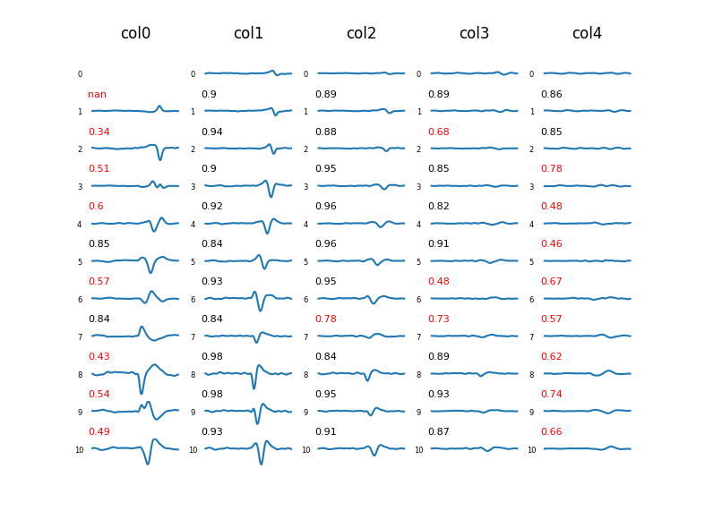
plot_muaps_for_cv(sta_dict, xcc_sta_dict, title='MUAPs for CV', figsize=[20, 15], tight_layout=False, line2d_kwargs_ax1=None, showimmediately=True)

Visualise MUAPs on which to calculate MUs CV.

Plot MUAPs obtained from the STA of the double differential signal and their paired cross-correlation value.

PARAMETER	DESCRIPTION
sta_dict	dict containing the STA of the double-differential derivation of a specific MU. TYPE: dict
xcc_sta_dict	dict containing the normalised cross-correlation coefficient of the double-differential derivation of a specific MU. TYPE: dict
title	Title of the plot. TYPE: str DEFAULT: "MUAPs from STA"
figsize	Size of the figure in centimeters [width, height]. TYPE: list DEFAULT: [20, 15]
tight_layout	If True (default), the plt.tight_layout() is called and the figure's layout is improved. It is useful to set it to False when calling the function from a GUI or if the final layout is not correct. TYPE: bool DEFAULT: False
line2d_kwargs_ax1	User-specified keyword arguments for sets of Line2D objects. This can be a list of dictionaries containing the kwargs for each Line2D, or a single dictionary. If a single dictionary is passed, the same style will be applied to all the lines. See examples. TYPE: dict or list DEFAULT: None
showimmediately	If True (default), plt.show() is called and the figure showed to the user. It is useful to set it to False when calling the function from a GUI. TYPE: bool DEFAULT: True

RETURNS	DESCRIPTION
fig	TYPE: pyplot `~.figure.Figure`

Examples:

Plot the double differential derivation and the XCC of adjacent channels for the first MU (0).

>>> import openhdemg.library as emg
>>> emgfile = emg.emg_from_samplefile()
>>> emgfile = emg.filter_rawemg(emgfile)
>>> sorted_rawemg = emg.sort_rawemg(
...     emgfile,
...     code="GR08MM1305",
...     orientation=180,
...     dividebycolumn=True
... )
>>> dd = emg.double_diff(sorted_rawemg)
>>> sta = emg.sta(
...     emgfile=emgfile,
...     sorted_rawemg=dd,
...     firings=[0, 50],
...     timewindow=50,
... )
>>> xcc_sta = emg.xcc_sta(sta)
>>> fig = emg.plot_muaps_for_cv(
...     sta_dict=sta[0],
...     xcc_sta_dict=xcc_sta[0],
...     showimmediately=True,
... )

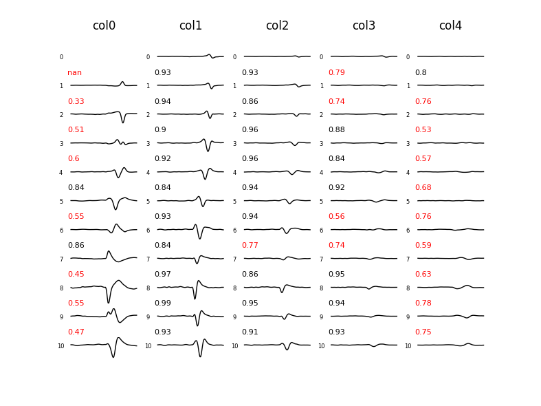
Customise the look of the plot.

>>> import openhdemg.library as emg
>>> emgfile = emg.emg_from_samplefile()
>>> emgfile = emg.filter_rawemg(emgfile)
>>> sorted_rawemg = emg.sort_rawemg(
...     emgfile,
...     code="GR08MM1305",
...     orientation=180,
...     dividebycolumn=True
... )
>>> dd = emg.double_diff(sorted_rawemg)
>>> sta = emg.sta(
...     emgfile=emgfile,
...     sorted_rawemg=dd,
...     firings="all",
...     timewindow=50,
... )
>>> xcc_sta = emg.xcc_sta(sta)
>>> line2d_kwargs_ax1 = {
...     "color": "k",
...     "linewidth": 1,
... }
>>> fig = emg.plot_muaps_for_cv(
...     sta_dict=sta[0],
...     xcc_sta_dict=xcc_sta[0],
...     line2d_kwargs_ax1=line2d_kwargs_ax1,
...     showimmediately=True,
... )

For further examples on how to customise the figure's layout, refer to plot_muaps().